Lecture 4: Parallel Programming Basics 📚¶

Parallel Programming Models 🖥️¶

1. Shared Address Space¶

• Communication: Implicit via loads/stores (unstructured).
• Pros: Natural programming model.
• Cons: Risk of poor performance due to unstructured communication.
• Example:
  
  C

  // Threads access shared variables directly
  float* A = allocate_shared(N);
  A[i] = A[j] + 1; // No explicit communication
  

2. Message Passing¶

• Communication: Explicit via send/receive.
• Pros: Structured communication aids scalability.
• Cons: Harder to implement initially.
• Example:
  
  C

  send(buffer, dest); // Explicit message
  recv(buffer, src);  // Explicit receive
  

3. Data Parallel¶

• Structure: Map operations over collections (e.g., arrays).
• Limitation: Restricted inter-iteration communication.
• Modern Use: CUDA/OpenCL allow limited shared-memory sync.

Hybrid Models 🌐¶

• Shared memory within a node + message passing between nodes.
• Example: MPI + OpenMP.

---

Example Applications 🌊¶

Ocean Current Simulation¶

• Grid-based 3D discretization:
• Dependencies within a single time step:
  
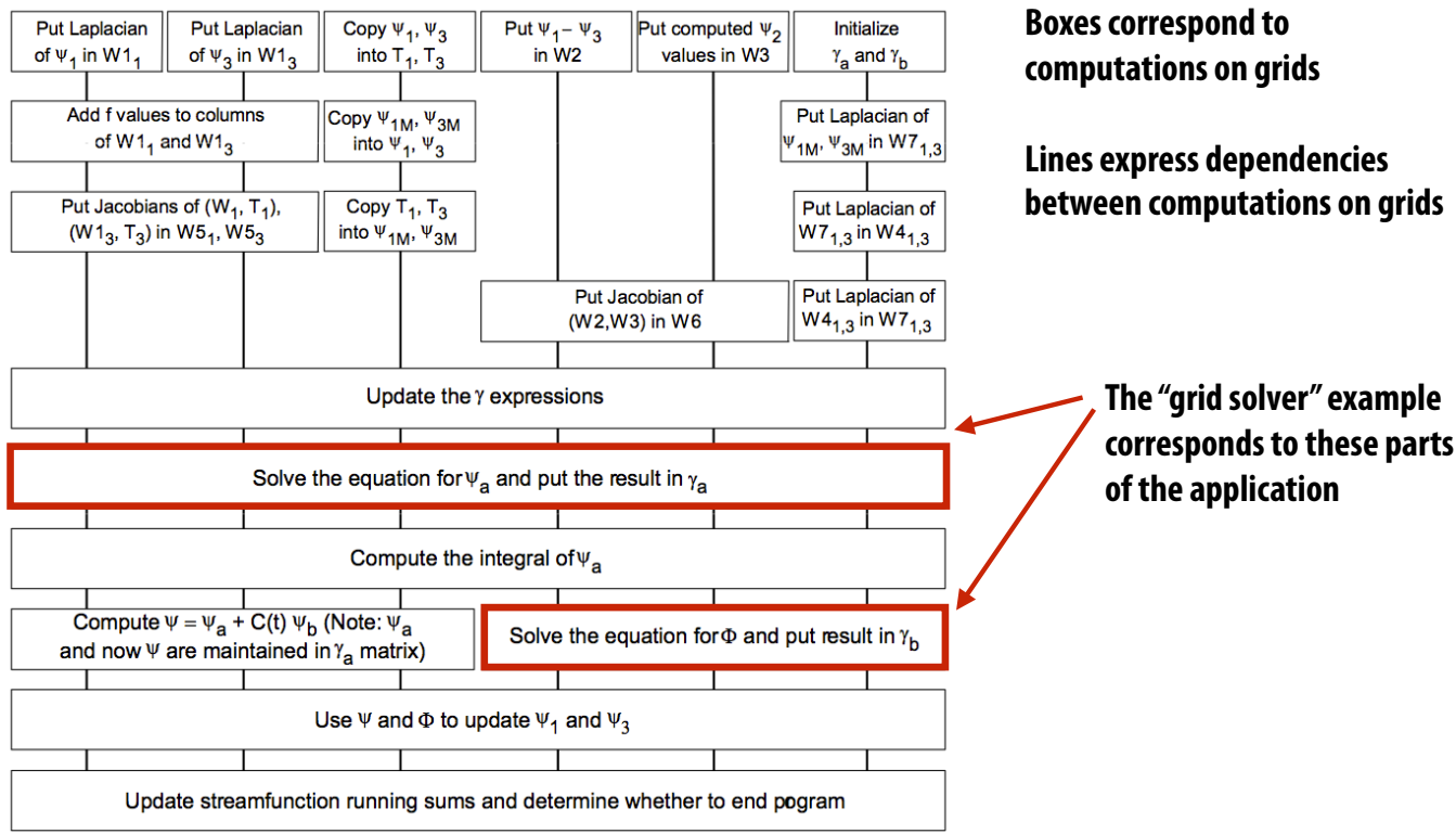
• Exploit data parallelism within grids.

Galaxy Evolution (Barnes-Hut Algorithm) 🌌¶

• N-body problem with \(O(N \log N)\) complexity.
• Quad-tree spatial decomposition:
  
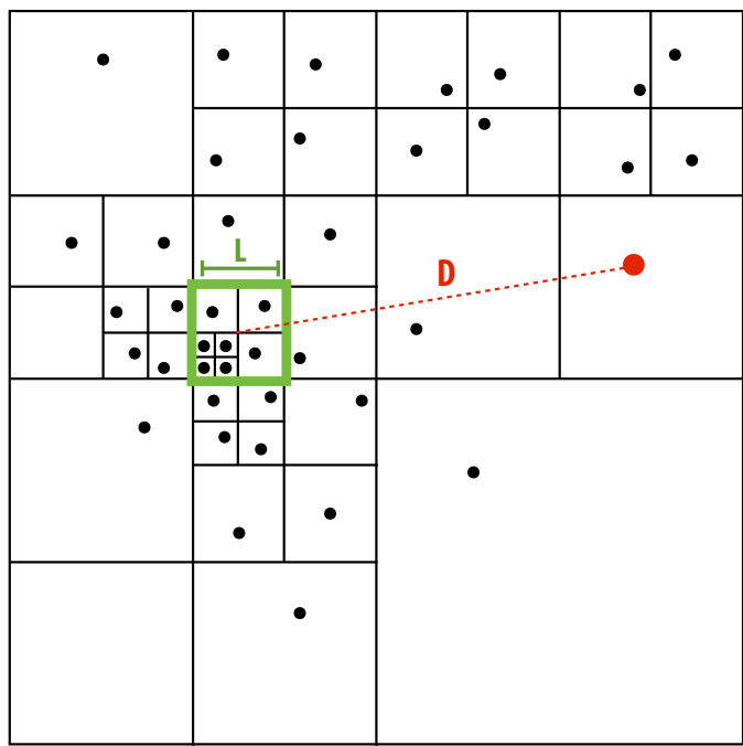
• Approximate far-field forces using aggregate mass in tree nodes.

---

Creating a Parallel Program 🛠️¶

Key Steps:¶

1. Decomposition: Break into parallel tasks.
2. Assignment: Map tasks to workers (threads/cores).
3. Orchestration: Manage sync, communication, and data locality.

Amdahl's Law ⚖️¶

• Formula:
  \(\(\text{Speedup} \leq \frac{1}{S + \frac{(1-S)}{P}}\)\)
• \(S\): Fraction of serial work.
• Example:
• Step 1 (parallel): \(N^2/P\) time.
• Step 2 (serial): \(N^2\) time.
• Speedup \(\leq 2\) for \(P\) processors if Step 2 remains serial.

---

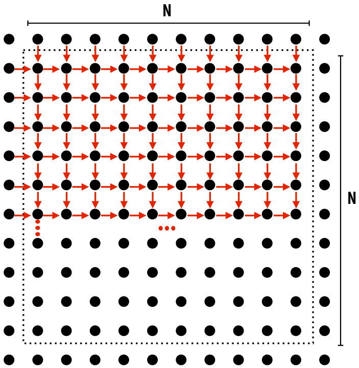
Case Study: 2D Grid Solver 🔢¶

Gauss-Seidel Iteration¶

• Sequential Code:
  
  C

  while (!done) {
    diff = 0;
    for (i, j) in grid {
      prev = A[i][j];
      A[i][j] = 0.2*(A[i-1][j] + A[i][j-1] + ...);
      diff += abs(A[i][j] - prev);
    }
    if (diff/N² < TOL) done = true;
  }
  

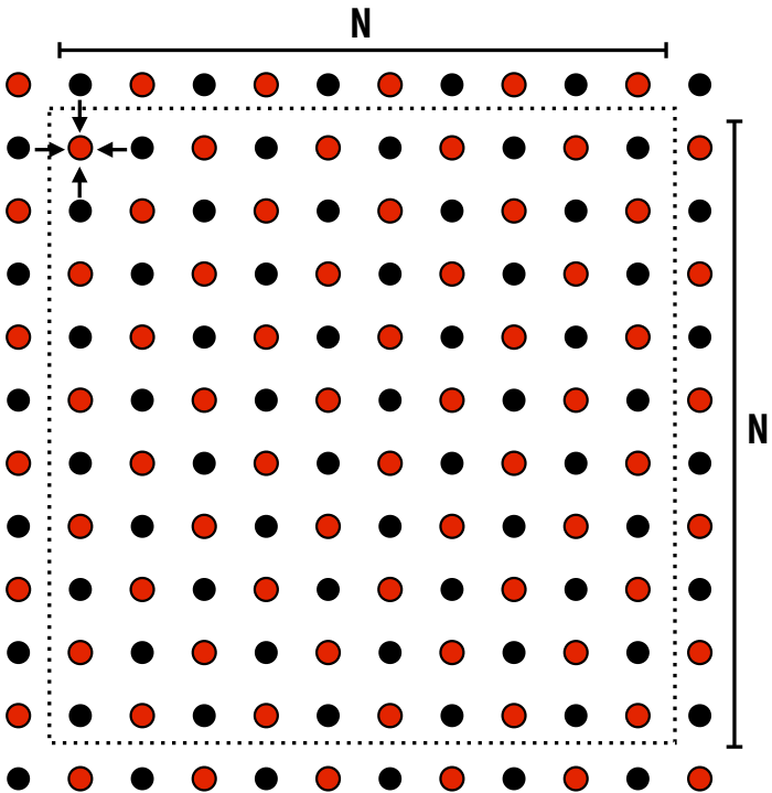
Parallelization Challenges ⚠️¶

• Dependencies:
  
• Solution: Red-Black Coloring 🎨
• Update all red cells → sync → update all black cells.
  

---

Synchronization Primitives 🔒¶

1. Locks¶

• Usage:
  
  C

  lock(myLock);
  critical_section();
  unlock(myLock);
  

2. Barriers¶

• Usage:
  
  C

  compute_phase1();
  barrier(all_threads);
  compute_phase2();
  

3. Message Passing¶

• Deadlock Avoidance:
  
  C

  if (tid % 2 == 0) {
    sendUp(); recvUp(); // Even threads send first
  } else {
    recvUp(); sendUp(); // Odd threads receive first
  }
  

---

Assignment Strategies 📋¶

Static vs. Dynamic¶

• Blocked Assignment:
• Thread 1: Rows 1–100; Thread 2: Rows 101–200.
• Interleaved Assignment:
• Thread 1: Rows 1, 3, 5...; Thread 2: Rows 2, 4, 6...

Performance Trade-offs¶

• Blocked: Better locality, less communication.
• Interleaved: Better load balance for irregular workloads.

---

Summary 📌¶

• Amdahl's Law limits speedup based on serial fractions.
• Decomposition is key to exposing parallelism.
• Hybrid Models (shared memory + message passing) dominate practice.
• Synchronization must balance correctness and overhead.

🚀 Next Lecture: CUDA/OpenCL for GPU parallelism!